Introduction
Innervate is a small neural-network library I wrote from scratch in Python and NumPy. It was not originally meant to be a polished machine-learning package. It was the software half of a larger hardware project: train a small handwritten-digit classifier, export the trained weights and biases, and then implement the resulting network on an FPGA through my VHDL hardware compiler, Innervator.
That background matters because the goal of this analysis is not simply “get the highest possible accuracy.” If that were the only goal, I would use a standard library model and be done. The more interesting question is whether a small, inspectable, from-scratch network can learn enough structure from handwritten digits to justify exporting its parameters to hardware.
The short answer is yes, but with caveats. On a larger stratified holdout set, the from-scratch network reaches 92.5% accuracy. That is good enough to show that the implementation learned real structure. It is not good enough to pretend that this is the best classifier for the dataset. Simple scikit-learn reference models do better. Fixed-point compression also costs accuracy, which is exactly the kind of hardware/software tradeoff the original project was meant to expose.
What this analysis is trying to prove
This report is not trying to prove that my from-scratch network is the best possible classifier for handwritten digits. It is not. A standard library model does better, and the reference models below make that clear.
The question is narrower and, for this project, more interesting:
- Can the original 64→20→10 network learn real digit structure on a larger and more defensible holdout set?
- Does it fail in interpretable ways, or does it merely produce arbitrary-looking mistakes?
- What accuracy is lost when the trained floating-point parameters are compressed toward the fixed-point format needed by the hardware implementation?
Those are the relevant questions because Innervate was never only a software exercise. It was the training/export half of Innervator, whose point was to turn a trained neural network into deterministic FPGA logic rather than leave it as another Python object.
Relevance to the application
The position I am using for this application is not a generic data-science job. It is a Ph.D. path in Electrical Engineering. That changes what counts as relevant. A purely black-box classifier would be less useful here than an analysis that connects learning, numerical representation, hardware constraints, and signal/image interpretation.
For that reason, I chose Innervate rather than a newer homework notebook. It lets me show a small but complete pipeline: data preprocessing, model training, validation, error analysis, comparison against reference models, and fixed-point compression for hardware export. That is much closer to the kind of boundary I am interested in: where algorithms stop being only software and start becoming physical implementations.
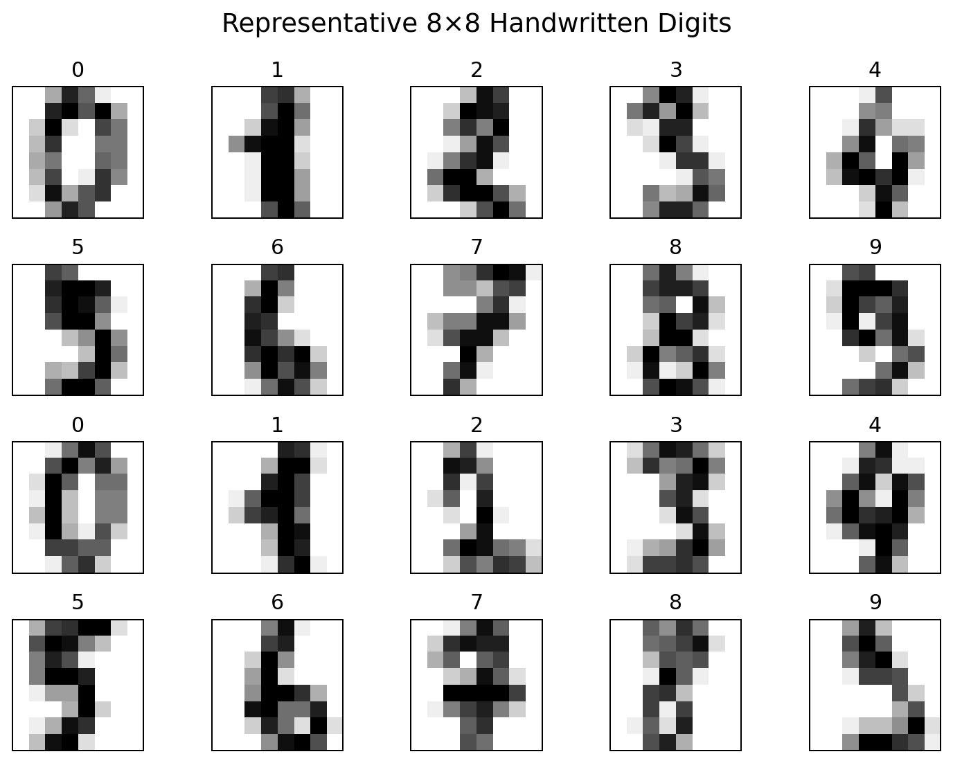
Data: 8×8 handwritten digits, not full MNIST
MNIST usually refers to the classic handwritten-digit recognition task: classify an image of a handwritten digit as 0, 1, 2, …, or 9. The famous version uses 28×28 grayscale images.
Strictly speaking, this project does not use canonical MNIST. It uses the smaller 8×8 handwritten-digits dataset. I sometimes call it “MNIST-8” as project shorthand, but the distinction matters: this is not the same benchmark, and its 64-pixel representation throws away a great deal of stroke detail.
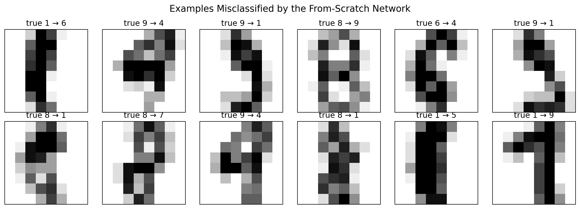
That changes the modeling problem. A 28×28 image has 784 pixels. An 8×8 image has only 64 pixels. This makes the problem small enough for a simple educational neural network and later FPGA implementation, but it also removes a lot of visual information. Some mistakes are therefore not surprising: at 8×8 resolution, a sloppy 8 can look like a 1, 3, 5, 6, 7, or 9.
The attached dataset contains two arrays:
| Object | Meaning | Shape |
|---|---|---|
data |
Flattened 8×8 grayscale images | 1,797 × 64 |
target |
True digit label from 0 through 9 | 1,797 |
The pixel intensities range from 0 to 16. There are no missing pixel values and no missing labels.
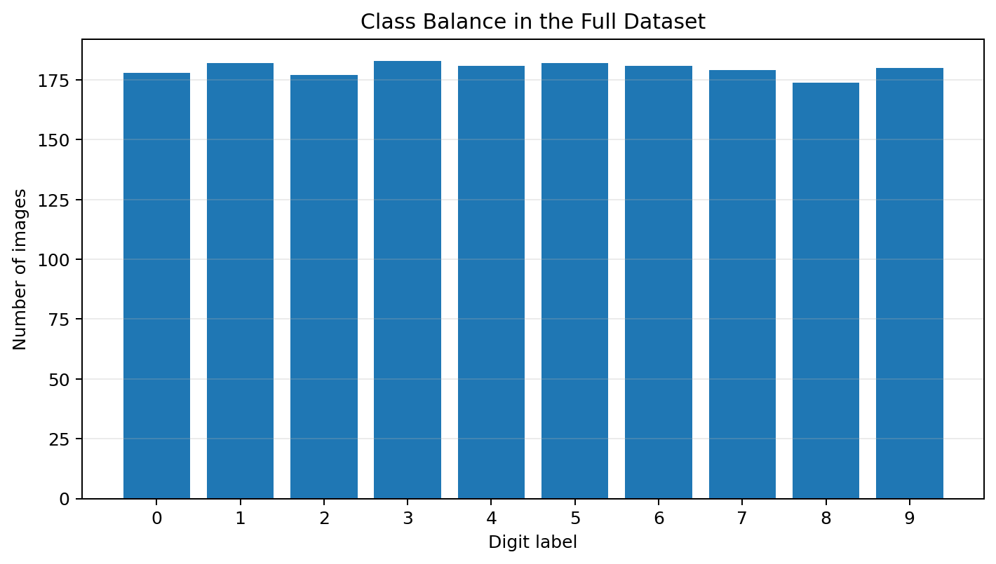
The class balance is also reasonable. Each digit appears between 174 and 183 times in the full dataset, so accuracy is not being inflated by one dominant class.
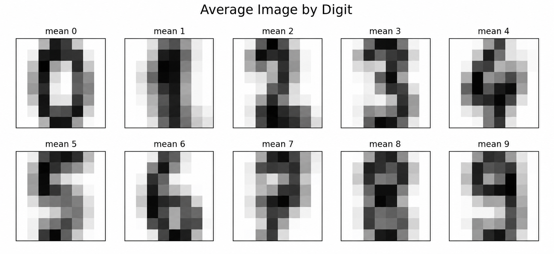
The average images are a quick sanity check before modeling. This is not a classifier, but it tells me whether the predictors contain class-specific signal. They do: zeros have a loop, ones are narrow, fours and sevens have stronger upper structure, and eights are denser near the middle.
Preprocessing
Preprocessing is done with these three commands:
images = images.reshape(images.shape[0], 8 * 8, 1)
images = images.astype("float32") / 15
labels = np.eye(10)[labels].reshape(labels.shape[0], 10, 1)
First, each 8×8 image is reshaped into a 64×1 column vector. Second, the pixel values are scaled. Third, each label is converted into a one-hot vector, so digit 3 becomes [0, 0, 0, 1, 0, 0, 0, 0, 0, 0].
I kept the original /15 scaling for the from-scratch network because the old project was written around a 4-bit grayscale assumption. However, the actual dataset includes pixel value 16. That means a few scaled pixel values become slightly larger than 1. I do not think that changes the main conclusion, but it is worth mentioning.
For the scikit-learn reference models, I used the more conventional raw_pixels / 16.0 scaling. I did this because those models are not part of the original hardware-export path; they are only reference points for how hard the classification problem is.
Validation split
The original project trained on the first 1,747 images and tested on the final 50. That was fine for a quick demonstration, but it is too fragile for a serious sample analysis. With only 50 test images, one mistake moves the accuracy by 2 percentage points. The final-50 split is also not evenly balanced: for example, it contains only 2 zeros but 7 fours.
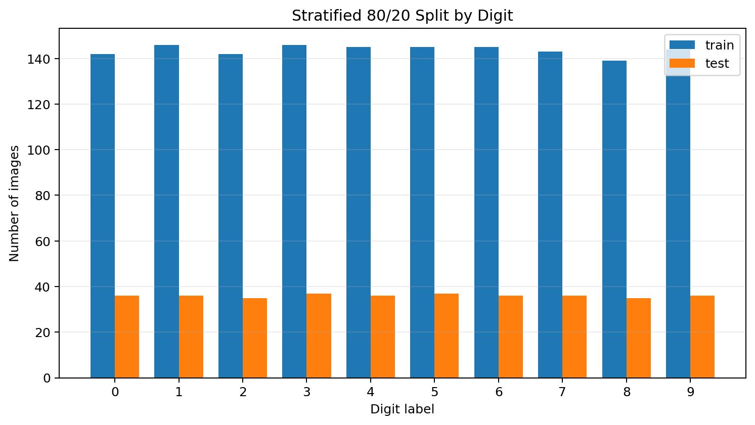
For the main evaluation, I therefore use a stratified 80/20 split:
| Split | Images | Purpose |
|---|---|---|
| Training | 1,437 | Fit the from-scratch network and reference models |
| Holdout | 360 | Estimate performance on images not used for training |
Stratification matters because this is a ten-class problem. I want every digit represented in the holdout set rather than letting the split accidentally overrepresent some digits and underrepresent others.
Model
The main model is the original Innervate dense neural network:
64 pixels (inputs) → 20 sigmoid hidden units → 10 sigmoid output units
Each dense layer applies an affine transformation and then a sigmoid activation:
\[\hat{y} = \sigma(Wx + b)\]The network has 1,510 trainable parameters.
| Layer | Weights | Biases | Total |
|---|---|---|---|
| Input → hidden | 64 × 20 = 1,280 | 20 | 1,300 |
| Hidden → output | 20 × 10 = 200 | 10 | 210 |
| Total | 1,480 | 30 | 1,510 |
The model is intentionally small. A larger network might improve accuracy, but that would weaken the connection to the hardware project. The point is to keep the forward pass, backpropagation, parameter export, and fixed-point compression simple enough to inspect at a glance.
Model-selection sanity check
The original project used a 64→20→10 network, 100 epochs, and learning rate 0.01. I did not want to silently inherit those choices and pretend they were tuned. So, before touching the final holdout set, I used the training portion only and carved out a small validation split to check a few nearby alternatives.
The point here was not to run an enormous hyperparameter search. That would be overkill for a 1,797-image educational dataset and would also move the project away from its hardware motivation. I only wanted to check whether the original configuration was at least reasonable.
| Hidden units | Learning rate | Epochs | Validation accuracy | Comment |
|---|---|---|---|---|
| 10 | 0.010 | 100 | 78.1% | Smaller, but not expressive enough |
| 20 | 0.003 | 100 | 78.5% | More cautious updates, but too slow here |
| 20 | 0.010 | 100 | 93.1% | Original configuration |
| 20 | 0.030 | 100 | 94.1% | Stronger validation score, but a less conservative update rule |
| 30 | 0.010 | 100 | 94.8% | Stronger validation score, but larger and less hardware-friendly |
A slightly larger or more aggressively trained network can do better as a classifier. I still keep the 20-hidden-unit model because the purpose of the project is not only classification. The 64→20→10 network is small, readable, and directly tied to the later FPGA implementation.
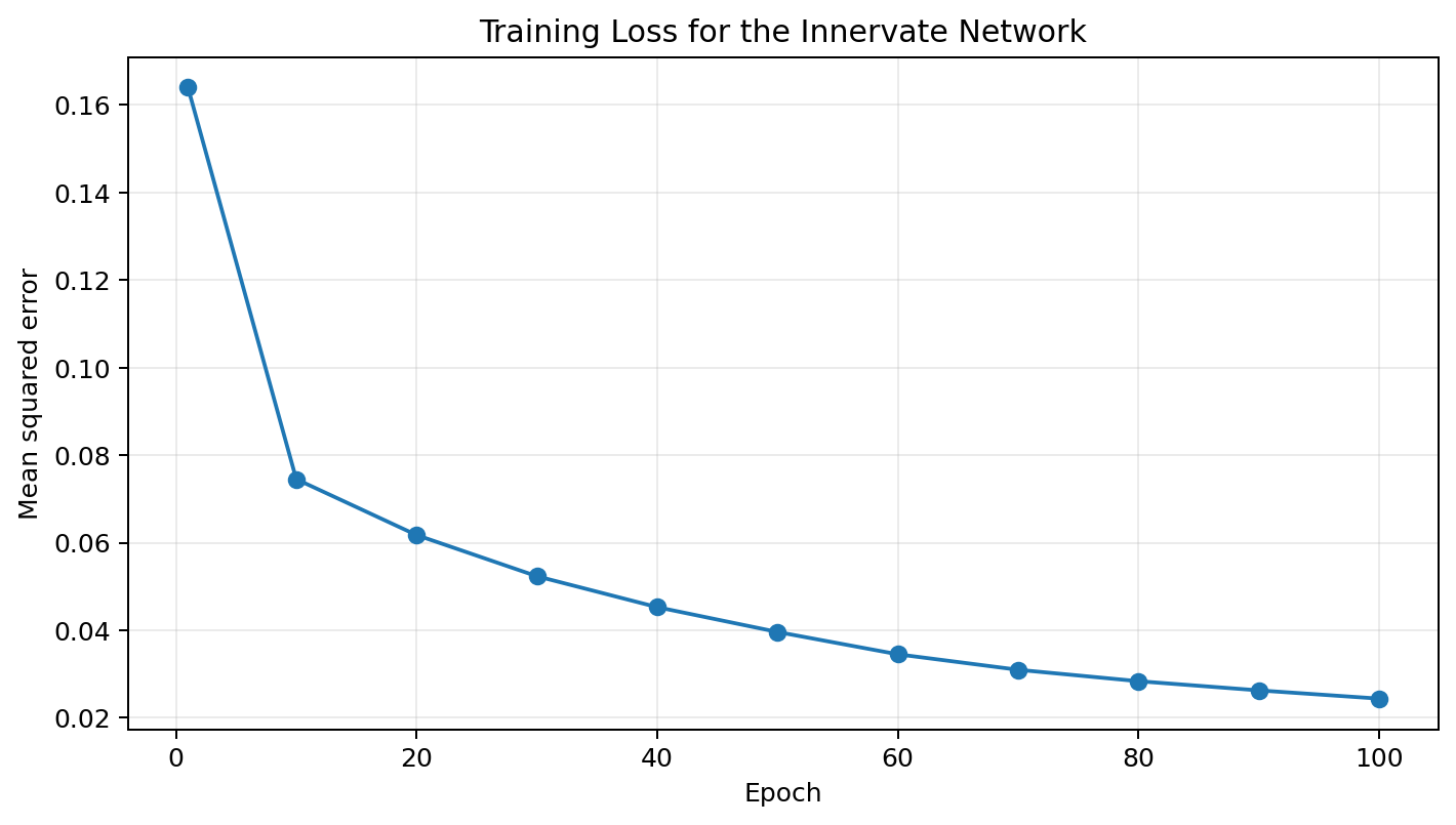
Training behavior
I retrained the network for 100 epochs with learning rate 0.01, matching the original project’s simple setup. The loss decreases steadily, which is a basic check that the network is learning a useful rule rather than producing random predictions.
Main results
| Evaluation | Images | Accuracy |
|---|---|---|
| Original saved model, original final-50 holdout | 50 | 92.0% |
Retrained Innervate, stratified training set |
1,437 | 92.8% |
Retrained Innervate, stratified holdout set |
360 | 92.5% |
Retrained Innervate after Q3.4 compression, stratified holdout |
360 | 88.9% |
The larger holdout confirms the basic story. The from-scratch model is not merely memorizing the training data: training accuracy and holdout accuracy are close. That said, I do not read 92.5% as “excellent” in the abstract. It is good for a small educational network, but it is not the best possible model for this dataset.
The confusion matrix shows the main weakness.
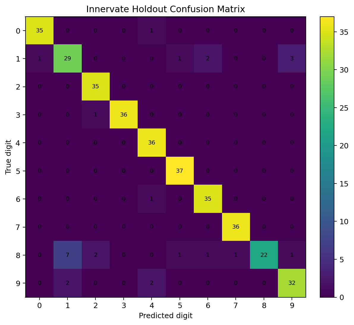
The per-class metrics make this more explicit.
| Digit | Support | Precision | Recall | F1 |
|---|---|---|---|---|
| 0 | 36 | 0.972 | 0.972 | 0.972 |
| 1 | 36 | 0.763 | 0.806 | 0.784 |
| 2 | 35 | 0.921 | 1.000 | 0.959 |
| 3 | 37 | 1.000 | 0.973 | 0.986 |
| 4 | 36 | 0.900 | 1.000 | 0.947 |
| 5 | 37 | 0.949 | 1.000 | 0.974 |
| 6 | 36 | 0.921 | 0.972 | 0.946 |
| 7 | 36 | 0.973 | 1.000 | 0.986 |
| 8 | 35 | 1.000 | 0.629 | 0.772 |
| 9 | 36 | 0.889 | 0.889 | 0.889 |
Digit 8 is the main problem. The model is conservative about predicting 8: when it predicts 8, it is right, but it misses many true 8s. That is why precision is high but recall is low. This is more informative than accuracy alone because it tells me where the classifier is failing.
There are at least two explanations for the digit-8 failure mode. The first is a data-resolution explanation: at 8×8 resolution, an 8 can genuinely collapse into something that looks like a 3, 5, 6, 9, or even a thick 1. The second is a model-capacity explanation: the network may not be learning enough local shape invariance, so it recognizes the easiest “canonical” eights but misses distorted ones.
The reference models help separate those explanations. Since 3-nearest neighbors does much better on the same split, the information is not completely absent from the data. Some of the problem is therefore not just resolution; it is also the particular representation learned by the small 64→20→10 sigmoid network.
Reference models
I also fit two ordinary scikit-learn models on the same stratified split. They are sanity checks; a sample analysis should not evaluate a custom model in a vacuum.
| Model | Holdout accuracy |
|---|---|
Innervate 64→20→10 DNN |
92.5% |
Innervate after Q3.4 compression |
88.9% |
| Logistic regression reference | 95.6% |
| 3-nearest-neighbor reference | 98.6% |
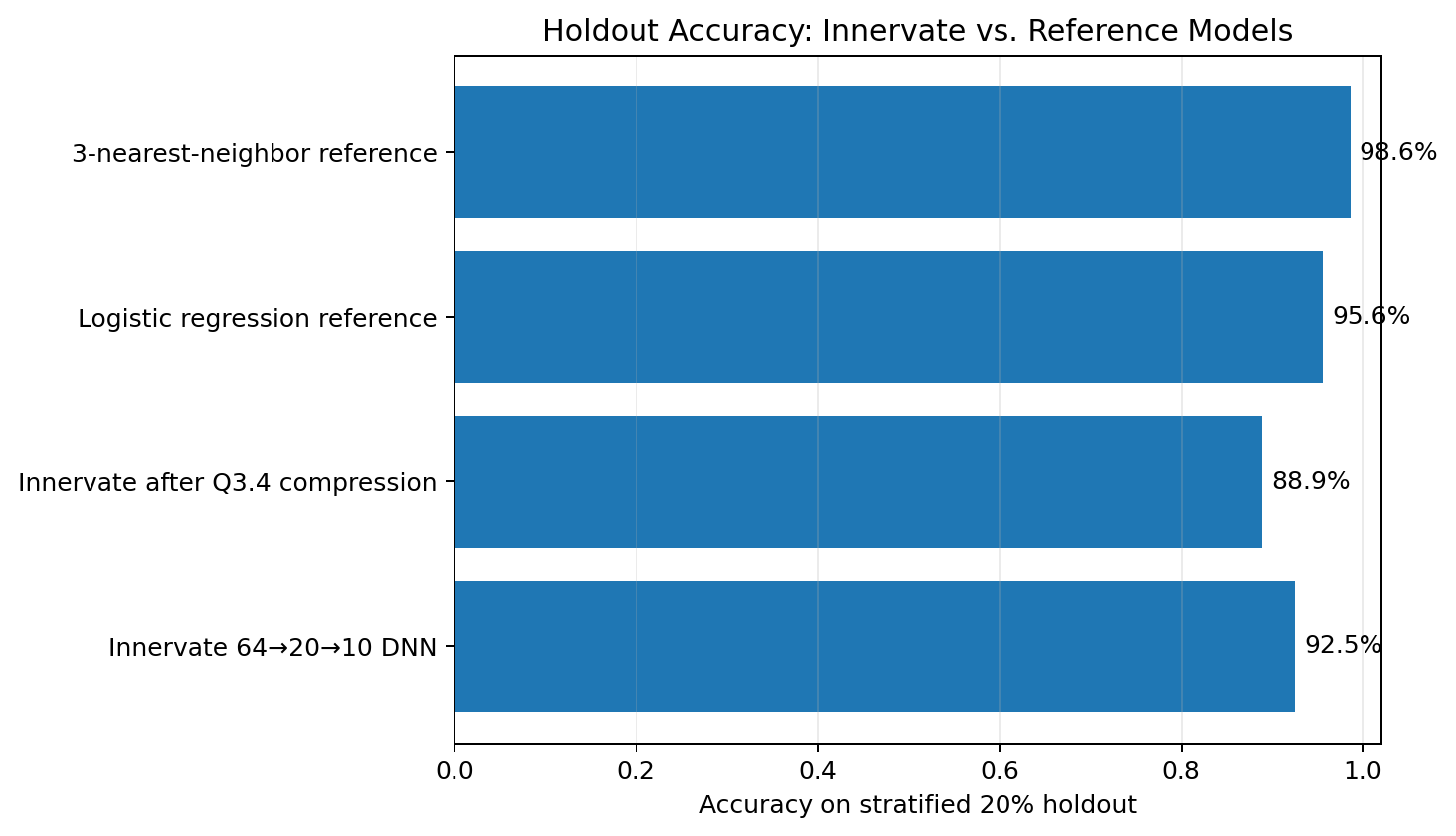
This comparison is important. I do not want the page to read like a sales pitch. The from-scratch network is useful because it exposes the mechanics of training and hardware export. It is not the best classifier here. The k-nearest-neighbor result is especially telling: for small grayscale digit images, comparing a test image to nearby training images is already a very strong strategy.
Confidence and error margins
The output layer uses sigmoid units rather than a softmax, so I do not treat the outputs as calibrated probabilities. Still, the gap between the largest output and the runner-up output is a useful confidence proxy.
| Outcome | Images | Mean margin | Median margin |
|---|---|---|---|
| Correct | 333 | 0.503 | 0.537 |
| Incorrect | 27 | 0.097 | 0.044 |
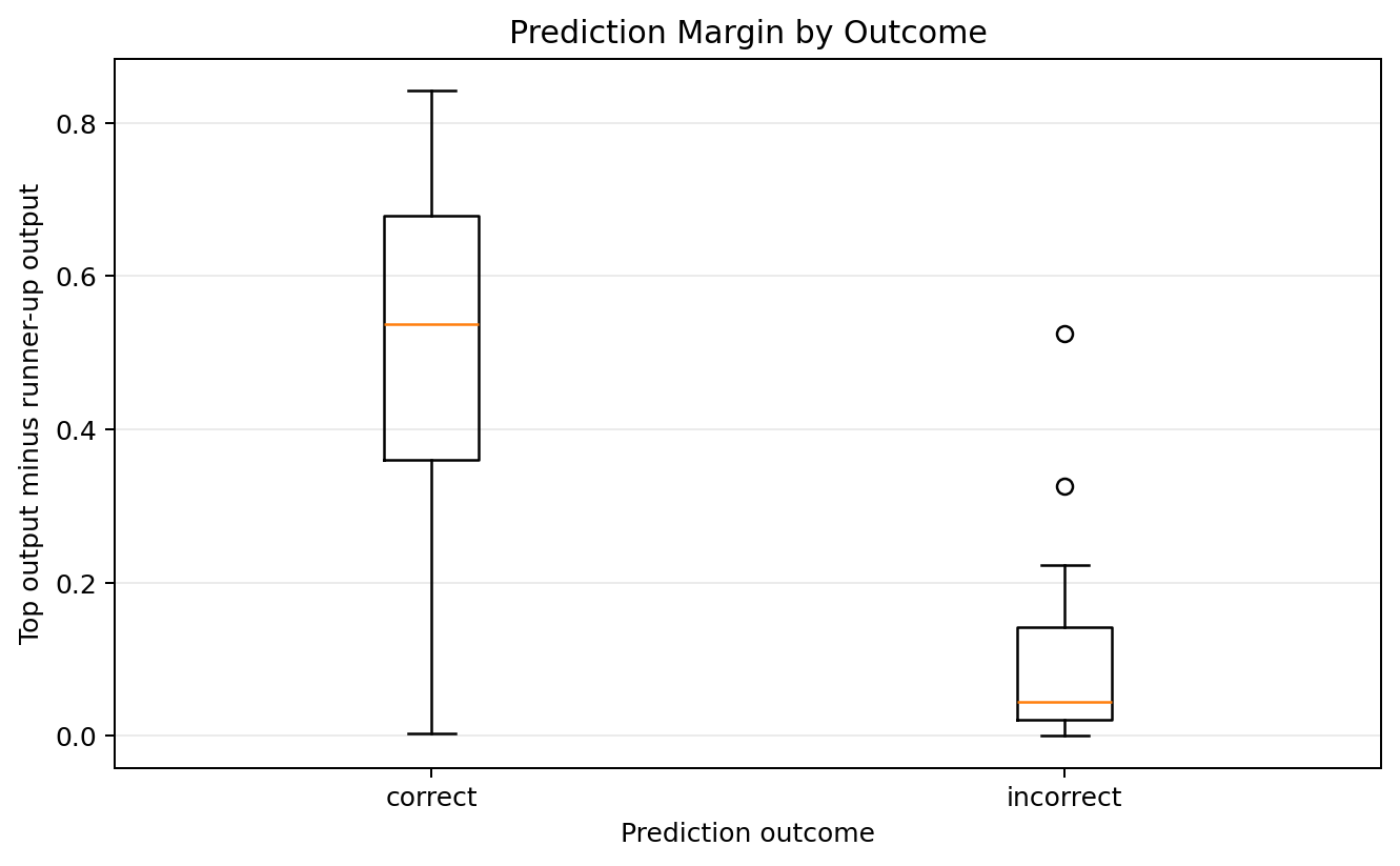
A deployed system could reject or flag low-margin predictions rather than forcing a digit classification every time. That would trade coverage for reliability.
Hardware-oriented compression audit
The hardware motivation is the most distinctive part of the project. The FPGA implementation cannot use arbitrary Python floats as-is. The old workflow therefore compressed weights and biases toward fixed-point values before export.
In the retrained model, I tested Q3.n-style compression by clipping values to the representable signed range and rounding them to different fractional resolutions.
| Fractional bits in Q3.n compression | Holdout accuracy |
|---|---|
| Uncompressed | 92.5% |
| 1 | 76.7% |
| 2 | 89.2% |
| 3 | 88.1% |
| 4 | 88.9% |
| 5 | 90.3% |
| 6 | 89.4% |
| 8 | 89.4% |
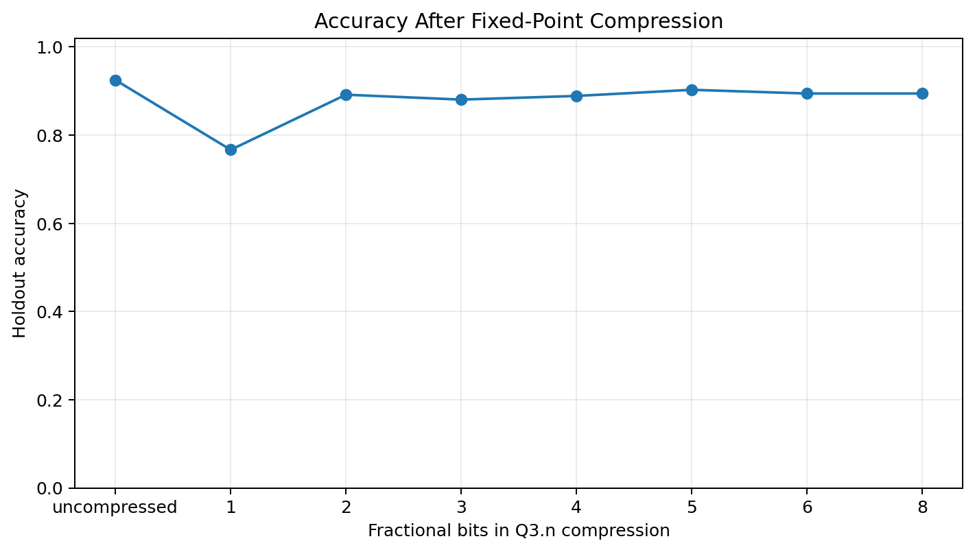
The result is not perfectly monotonic because the model was not trained with quantization in the loop. Rounding can move borderline predictions in either direction.
A pure accuracy table is useful, but it does not say much about why compression hurts. So I also checked how much the parameter values actually moved under compression.
| Compression | Max absolute parameter change | Mean absolute parameter change | Parameters clipped | Holdout accuracy |
|---|---|---|---|---|
| Q3.1 | 22.412 | 0.163 | 8 / 1,510 | 76.7% |
| Q3.2 | 22.412 | 0.101 | 8 / 1,510 | 89.2% |
| Q3.4 | 22.412 | 0.055 | 8 / 1,510 | 88.9% |
| Q3.8 | 22.412 | 0.040 | 8 / 1,510 | 89.4% |
The maximum change is dominated by a small number of clipped parameters. The mean change is more representative of the whole network, and it falls as the number of fractional bits increases. Still, the clipping result matters: even if only 8 out of 1,510 parameters exceed the Q3 range, those parameters can affect decision boundaries.
Interpretation and limitations
The project passes the main sanity checks. The model learns real structure, the larger holdout split gives a more credible estimate than the original final-50 test, and the errors are interpretable rather than random.
The limitations are just as important:
- the original 50-image holdout was too small for a serious performance claim;
- the code uses sigmoid + mean-squared error rather than the more standard softmax + cross-entropy setup;
- the backpropagation implementation has a gradient-propagation caveat;
- the
/15scaling reflects the old code’s 4-bit assumption even though the dataset includes pixel value 16; - fixed-point compression should ideally be considered during training, not only after training;
- the validation check suggests that a slightly larger or more aggressively trained network could improve accuracy; and
- standard scikit-learn reference models outperform the from-scratch network on this dataset.
I would improve the project by fixing the backpropagation implementation, switching the classifier head to softmax with cross-entropy, using train/validation/test splits for actual hyperparameter tuning, and adding quantization-aware training before exporting to FPGA hardware.
I would also separate two goals more cleanly in a future version. If the goal is maximum classification accuracy, then I should use the strongest small model I can justify. If the goal is hardware export and interpretability, then the smaller 64→20→10 network is still defensible, but the performance claim should be made with that constraint clearly stated. This report takes the second path.
Conclusion
Innervate is not the strongest possible digit classifier. That is not the point. It is a compact, auditable neural-network implementation that let me connect machine learning and hardware constraints in one project.
The main result is that the from-scratch 64→20→10 network reaches 92.5% holdout accuracy on a stratified 360-image test set. That is enough to show that the implementation learned real digit structure, but the reference models and compression audit keep the claim honest.
The best summary is this: Innervate works as a small educational neural-network implementation and as a bridge to Innervator; it should not be mistaken for a state-of-the-art digit-recognition system.
Reproducibility
The website artifacts were generated with:
python scripts/evaluate_innervate.py
The script reloads the dataset, retrains the Innervate network on the stratified split, regenerates all figures, writes the CSV files in assets/data, and repeats the fixed-point compression audit. Running the script should recreate the files in assets/figures/ and assets/data/. The generated values may differ if the random seed is changed, so the script fixes the seed used for the reported website results.
Dependencies:
python -m pip install -r requirements.txt
The source ZIP below includes the original Innervate code used for the main model. The scikit-learn models are only reference models; they are not used for the main from-scratch classifier.